| Model |
Top-1 Accuracy (%) |
GPU Inference Time (ms) |
CPU Inference Time (ms) |
Model Size (M) |
Description |
| CLIP_vit_base_patch16_224 |
85.36 |
13.1957 |
285.493 |
306.5 M |
CLIP is an image classification model based on the correlation between vision and language. It adopts contrastive learning and pre-training methods to achieve unsupervised or weakly supervised image classification, especially suitable for large-scale datasets. By mapping images and texts into the same representation space, the model learns general features, exhibiting good generalization ability and interpretability. With relatively good training errors, it performs well in many downstream tasks. |
| CLIP_vit_large_patch14_224 |
88.1 |
51.1284 |
1131.28 |
1.04 G |
| ConvNeXt_base_224 |
83.84 |
12.8473 |
1513.87 |
313.9 M |
The ConvNeXt series of models were proposed by Meta in 2022, based on the CNN architecture. This series of models builds upon ResNet, incorporating the advantages of SwinTransformer, including training strategies and network structure optimization ideas, to improve the pure CNN architecture network. It explores the performance limits of convolutional neural networks. The ConvNeXt series of models possesses many advantages of convolutional neural networks, including high inference efficiency and ease of migration to downstream tasks. |
| ConvNeXt_base_384 |
84.90 |
31.7607 |
3967.05 |
313.9 M |
| ConvNeXt_large_224 |
84.26 |
26.8103 |
2463.56 |
700.7 M |
| ConvNeXt_large_384 |
85.27 |
66.4058 |
6598.92 |
700.7 M |
| ConvNeXt_small |
83.13 |
9.74075 |
1127.6 |
178.0 M |
| ConvNeXt_tiny |
82.03 |
5.48923 |
672.559 |
104.1 M |
| FasterNet-L |
83.5 |
23.4415 |
- |
357.1 M |
FasterNet is a neural network designed to improve runtime speed. Its key improvements are as follows:
1. Re-examined popular operators and found that low FLOPS mainly stem from frequent memory accesses, especially in depthwise convolutions;
2. Proposed Partial Convolution (PConv) to extract image features more efficiently by reducing redundant computations and memory accesses;
3. Launched the FasterNet series of models based on PConv, a new design scheme that achieves significantly higher runtime speeds on various devices without compromising model task performance. |
| FasterNet-M |
83.0 |
21.8936 |
- |
204.6 M |
| FasterNet-S |
81.3 |
13.0409 |
- |
119.3 M |
| FasterNet-T0 |
71.9 |
12.2432 |
- |
15.1 M |
| FasterNet-T1 |
75.9 |
11.3562 |
- |
29.2 M |
| FasterNet-T2 |
79.1 |
10.703 |
- |
57.4 M |
| MobileNetV1_x0_5 |
63.5 |
1.86754 |
7.48297 |
4.8 M |
MobileNetV1 is a network released by Google in 2017 for mobile devices or embedded devices. This network decomposes traditional convolution operations into depthwise separable convolutions, which are a combination of Depthwise convolution and Pointwise convolution. Compared to traditional convolutional networks, this combination can significantly reduce the number of parameters and computations. Additionally, this network can be used for image classification and other vision tasks. |
| MobileNetV1_x0_25 |
51.4 |
1.83478 |
4.83674 |
1.8 M |
| MobileNetV1_x0_75 |
68.8 |
2.57903 |
10.6343 |
9.3 M |
| MobileNetV1_x1_0 |
71.0 |
2.78781 |
13.98 |
15.2 M |
| MobileNetV2_x0_5 |
65.0 |
4.94234 |
11.1629 |
7.1 M |
MobileNetV2 is a lightweight network proposed by Google following MobileNetV1. Compared to MobileNetV1, MobileNetV2 introduces Linear bottlenecks and Inverted residual blocks as the basic structure of the network. By stacking these basic modules extensively, the network structure of MobileNetV2 is formed. Finally, it achieves higher classification accuracy with only half the FLOPs of MobileNetV1. |
| MobileNetV2_x0_25 |
53.2 |
4.50856 |
9.40991 |
5.5 M |
| MobileNetV2_x1_0 |
72.2 |
6.12159 |
16.0442 |
12.6 M |
| MobileNetV2_x1_5 |
74.1 |
6.28385 |
22.5129 |
25.0 M |
| MobileNetV2_x2_0 |
75.2 |
6.12888 |
30.8612 |
41.2 M |
| MobileNetV3_large_x0_5 |
69.2 |
6.31302 |
14.5588 |
9.6 M |
MobileNetV3 is a NAS-based lightweight network proposed by Google in 2019. To further enhance performance, relu and sigmoid activation functions are replaced with hard_swish and hard_sigmoid activation functions, respectively. Additionally, some improvement strategies specifically designed to reduce network computations are introduced. |
| MobileNetV3_large_x0_35 |
64.3 |
5.76207 |
13.9041 |
7.5 M |
| MobileNetV3_large_x0_75 |
73.1 |
8.41737 |
16.9506 |
14.0 M |
| MobileNetV3_large_x1_0 |
75.3 |
8.64112 |
19.1614 |
19.5 M |
| MobileNetV3_large_x1_25 |
76.4 |
8.73358 |
22.1296 |
26.5 M |
| MobileNetV3_small_x0_5 |
59.2 |
5.16721 |
11.2688 |
6.8 M |
| MobileNetV3_small_x0_35 |
53.0 |
5.22053 |
11.0055 |
6.0 M |
| MobileNetV3_small_x0_75 |
66.0 |
5.39831 |
12.8313 |
8.5 M |
| MobileNetV3_small_x1_0 |
68.2 |
6.00993 |
12.9598 |
10.5 M |
| MobileNetV3_small_x1_25 |
70.7 |
6.9589 |
14.3995 |
13.0 M |
| MobileNetV4_conv_large |
83.4 |
12.5485 |
51.6453 |
125.2 M |
MobileNetV4 is an efficient architecture specifically designed for mobile devices. Its core lies in the introduction of the UIB (Universal Inverted Bottleneck) module, a unified and flexible structure that integrates IB (Inverted Bottleneck), ConvNeXt, FFN (Feed Forward Network), and the latest ExtraDW (Extra Depthwise) module. Alongside UIB, Mobile MQA, a customized attention block for mobile accelerators, was also introduced, achieving up to 39% significant acceleration. Furthermore, MobileNetV4 introduces a novel Neural Architecture Search (NAS) scheme to enhance the effectiveness of the search process. |
| MobileNetV4_conv_medium |
79.9 |
9.65509 |
26.6157 |
37.6 M |
| MobileNetV4_conv_small |
74.6 |
5.24172 |
11.0893 |
14.7 M |
| MobileNetV4_hybrid_large |
83.8 |
20.0726 |
213.769 |
145.1 M |
| MobileNetV4_hybrid_medium |
80.5 |
19.7543 |
62.2624 |
42.9 M |
| PP-HGNet_base |
85.0 |
14.2969 |
327.114 |
249.4 M |
PP-HGNet (High Performance GPU Net) is a high-performance backbone network developed by Baidu PaddlePaddle's vision team, tailored for GPU platforms. This network combines the fundamentals of VOVNet with learnable downsampling layers (LDS Layer), incorporating the advantages of models such as ResNet_vd and PPHGNet. On GPU platforms, this model achieves higher accuracy compared to other SOTA models at the same speed. Specifically, it outperforms ResNet34-0 by 3.8 percentage points and ResNet50-0 by 2.4 percentage points. Under the same SLSD conditions, it ultimately surpasses ResNet50-D by 4.7 percentage points. Additionally, at the same level of accuracy, its inference speed significantly exceeds that of mainstream Vision Transformers. |
| PP-HGNet_small |
81.51 |
5.50661 |
119.041 |
86.5 M |
| PP-HGNet_tiny |
79.83 |
5.22006 |
69.396 |
52.4 M |
| PP-HGNetV2-B0 |
77.77 |
6.53694 |
23.352 |
21.4 M |
PP-HGNetV2 (High Performance GPU Network V2) is the next-generation version of Baidu PaddlePaddle's PP-HGNet, featuring further optimizations and improvements upon its predecessor. It pushes the limits of NVIDIA's "Accuracy-Latency Balance," significantly outperforming other models with similar inference speeds in terms of accuracy. It demonstrates strong performance across various label classification and evaluation scenarios. |
| PP-HGNetV2-B1 |
79.18 |
6.56034 |
27.3099 |
22.6 M |
| PP-HGNetV2-B2 |
81.74 |
9.60494 |
43.1219 |
39.9 M |
| PP-HGNetV2-B3 |
82.98 |
11.0042 |
55.1367 |
57.9 M |
| PP-HGNetV2-B4 |
83.57 |
9.66407 |
54.2462 |
70.4 M |
| PP-HGNetV2-B5 |
84.75 |
15.7091 |
115.926 |
140.8 M |
| PP-HGNetV2-B6 |
86.30 |
21.226 |
255.279 |
268.4 M |
| PP-LCNet_x0_5 |
63.14 |
3.67722 |
6.66857 |
6.7 M |
PP-LCNet is a lightweight backbone network developed by Baidu PaddlePaddle's vision team. It enhances model performance without increasing inference time, significantly surpassing other lightweight SOTA models. |
| PP-LCNet_x0_25 |
51.86 |
2.65341 |
5.81357 |
5.5 M |
| PP-LCNet_x0_35 |
58.09 |
2.7212 |
6.28944 |
5.9 M |
| PP-LCNet_x0_75 |
68.18 |
3.91032 |
8.06953 |
8.4 M |
| PP-LCNet_x1_0 |
71.32 |
3.84845 |
9.23735 |
10.5 M |
| PP-LCNet_x1_5 |
73.71 |
3.97666 |
12.3457 |
16.0 M |
| PP-LCNet_x2_0 |
75.18 |
4.07556 |
16.2752 |
23.2 M |
| PP-LCNet_x2_5 |
76.60 |
4.06028 |
21.5063 |
32.1 M |
| PP-LCNetV2_base |
77.05 |
5.23428 |
19.6005 |
23.7 M |
The PP-LCNetV2 image classification model is the next-generation version of PP-LCNet, self-developed by Baidu PaddlePaddle's vision team. Based on PP-LCNet, it has undergone further optimization and improvements, primarily utilizing re-parameterization strategies to combine depthwise convolutions with varying kernel sizes and optimizing pointwise convolutions, Shortcuts, etc. Without using additional data, the PPLCNetV2_base model achieves over 77% Top-1 Accuracy on the ImageNet dataset for image classification, while maintaining an inference time of less than 4.4 ms on Intel CPU platforms. |
| PP-LCNetV2_large |
78.51 |
6.78335 |
30.4378 |
37.3 M |
| PP-LCNetV2_small |
73.97 |
3.89762 |
13.0273 |
14.6 M |
| ResNet18_vd |
72.3 |
3.53048 |
31.3014 |
41.5 M |
The ResNet series of models were introduced in 2015, winning the ILSVRC2015 competition with a top-5 error rate of 3.57%. This network innovatively proposed residual structures, which are stacked to construct the ResNet network. Experiments have shown that using residual blocks can effectively improve convergence speed and accuracy. |
| ResNet18 |
71.0 |
2.4868 |
27.4601 |
41.5 M |
| ResNet34_vd |
76.0 |
5.60675 |
56.0653 |
77.3 M |
| ResNet34 |
74.6 |
4.16902 |
51.925 |
77.3 M |
| ResNet50_vd |
79.1 |
10.1885 |
68.446 |
90.8 M |
| ResNet50 |
76.5 |
9.62383 |
64.8135 |
90.8 M |
| ResNet101_vd |
80.2 |
20.0563 |
124.85 |
158.4 M |
| ResNet101 |
77.6 |
19.2297 |
121.006 |
158.4 M |
| ResNet152_vd |
80.6 |
29.6439 |
181.678 |
214.3 M |
| ResNet152 |
78.3 |
30.0461 |
177.707 |
214.2 M |
| ResNet200_vd |
80.9 |
39.1628 |
235.185 |
266.0 M |
| StarNet-S1 |
73.6 |
9.895 |
23.0465 |
11.2 M |
StarNet focuses on exploring the untapped potential of "star operations" (i.e., element-wise multiplication) in network design. It reveals that star operations can map inputs to high-dimensional, nonlinear feature spaces, a process akin to kernel tricks but without the need to expand the network size. Consequently, StarNet, a simple yet powerful prototype network, is further proposed, demonstrating exceptional performance and low latency under compact network structures and limited computational resources. |
| StarNet-S2 |
74.8 |
7.91279 |
21.9571 |
14.3 M |
| StarNet-S3 |
77.0 |
10.7531 |
30.7656 |
22.2 M |
| StarNet-S4 |
79.0 |
15.2868 |
43.2497 |
28.9 M |
| SwinTransformer_base_patch4_window7_224 |
83.37 |
16.9848 |
383.83 |
310.5 M |
SwinTransformer is a novel vision Transformer network that can serve as a general-purpose backbone for computer vision tasks. SwinTransformer consists of a hierarchical Transformer structure represented by shifted windows. Shifted windows restrict self-attention computations to non-overlapping local windows while allowing cross-window connections, thereby enhancing network performance. |
| SwinTransformer_base_patch4_window12_384 |
84.17 |
37.2855 |
1178.63 |
311.4 M |
| SwinTransformer_large_patch4_window7_224 |
86.19 |
27.5498 |
689.729 |
694.8 M |
| SwinTransformer_large_patch4_window12_384 |
87.06 |
74.1768 |
2105.22 |
696.1 M |
| SwinTransformer_small_patch4_window7_224 |
83.21 |
16.3982 |
285.56 |
175.6 M |
| SwinTransformer_tiny_patch4_window7_224 |
81.10 |
8.54846 |
156.306 |
100.1 M |
**Note: The above accuracy metrics refer to Top-1 Accuracy on the [ImageNet-1k](https://www.image-net.org/index.php) validation set. ****All model GPU inference times are based on NVIDIA Tesla T4 machines, with precision type FP32. CPU inference speeds are based on Intel® Xeon® Gold 5117 CPU @ 2.00GHz, with 8 threads and precision type FP32.**
III. Quick Integration
❗ Before quick integration, please install the PaddleX wheel package. For detailed instructions, refer to the PaddleX Local Installation Guide.
After installing the wheel package, you can complete image classification module inference with just a few lines of code. You can switch between models in this module freely, and you can also integrate the model inference of the image classification module into your project. Before running the following code, please download the demo image to your local machine.
from paddlex import create_model
model = create_model("PP-LCNet_x1_0")
output = model.predict("general_image_classification_001.jpg", batch_size=1)
for res in output:
    res.print(json_format=False)
    res.save_to_img("./output/")
    res.save_to_json("./output/res.json")
For more information on using PaddleX's single-model inference APIs, please refer to the PaddleX Single-Model Python Script Usage Instructions.
IV. Custom Development
If you are seeking higher accuracy from existing models, you can use PaddleX's custom development capabilities to develop better image classification models. Before using PaddleX to develop image classification models, please ensure that you have installed the relevant model training plugins for image classification in PaddleX. The installation process can be found in the custom development section of the PaddleX Local Installation Guide.
4.1 Data Preparation
Before model training, you need to prepare the dataset for the corresponding task module. PaddleX provides data validation functionality for each module, and only data that passes data validation can be used for model training. Additionally, PaddleX provides demo datasets for each module, which you can use to complete subsequent development. If you wish to use your own private dataset for subsequent model training, please refer to the PaddleX Image Classification Task Module Data Annotation Guide.
4.1.1 Demo Data Download
You can use the following command to download the demo dataset to a specified folder:
cd /path/to/paddlex
wget https://paddle-model-ecology.bj.bcebos.com/paddlex/data/cls_flowers_examples.tar -P ./dataset
tar -xf ./dataset/cls_flowers_examples.tar -C ./dataset/
4.1.2 Data Validation
One command is all you need to complete data validation:
python main.py -c paddlex/configs/image_classification/PP-LCNet_x1_0.yaml \
    -o Global.mode=check_dataset \
    -o Global.dataset_dir=./dataset/cls_flowers_examples
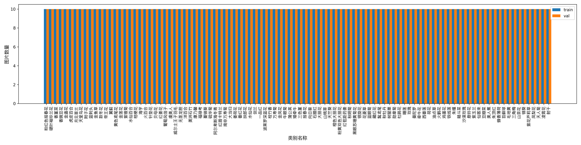
After executing the above command, PaddleX will validate the dataset and summarize its basic information. If the command runs successfully, it will print Check dataset passed ! in the log. The validation results file is saved in ./output/check_dataset_result.json, and related outputs are saved in the ./output/check_dataset directory in the current directory, including visual examples of sample images and sample distribution histograms.
👉 Validation Results Details (Click to Expand)
```bash
{
"done_flag": true,
"check_pass": true,
"attributes": {
"label_file": "dataset/label.txt",
"num_classes": 102,
"train_samples": 1020,
"train_sample_paths": [
"check_dataset/demo_img/image_01904.jpg",
"check_dataset/demo_img/image_06940.jpg"
],
"val_samples": 1020,
"val_sample_paths": [
"check_dataset/demo_img/image_01937.jpg",
"check_dataset/demo_img/image_06958.jpg"
]
},
"analysis": {
"histogram": "check_dataset/histogram.png"
},
"dataset_path": "./dataset/cls_flowers_examples",
"show_type": "image",
"dataset_type": "ClsDataset"
}
```
The above validation results, with check_pass being True, indicate that the dataset format meets the requirements. Explanations for other indicators are as follows:
* `attributes.num_classes`: The number of classes in this dataset is 102;
* `attributes.train_samples`: The number of training set samples in this dataset is 1020;
* `attributes.val_samples`: The number of validation set samples in this dataset is 1020;
* `attributes.train_sample_paths`: A list of relative paths to the visual samples in the training set of this dataset;
* `attributes.val_sample_paths`: A list of relative paths to the visual samples in the validation set of this dataset;
Additionally, the dataset validation analyzes the sample number distribution across all classes in the dataset and generates a distribution histogram (histogram.png):
4.1.3 Dataset Format Conversion/Dataset Splitting (Optional)
After completing data validation, you can convert the dataset format or re-split the training/validation ratio of the dataset by modifying the configuration file or appending hyperparameters.
👉 Dataset Format Conversion/Dataset Splitting Details (Click to Expand)
**(1) Dataset Format Conversion**
Image classification does not currently support data conversion.
**(2) Dataset Splitting**
The parameters for dataset splitting can be set by modifying the fields under `CheckDataset` in the configuration file. The following are example explanations for some of the parameters in the configuration file:
* `CheckDataset`:
* `split`:
* `enable`: Whether to re-split the dataset. When set to `True`, the dataset format will be converted. The default is `False`;
* `train_percent`: If re-splitting the dataset, you need to set the percentage of the training set, which should be an integer between 0-100, ensuring that the sum with `val_percent` equals 100;
For example, if you want to re-split the dataset with a 90% training set and a 10% validation set, you need to modify the configuration file as follows:
```bash
......
CheckDataset:
......
split:
enable: True
train_percent: 90
val_percent: 10
......
```
Then execute the command:
```bash
python main.py -c paddlex/configs/image_classification/PP-LCNet_x1_0.yaml \
-o Global.mode=check_dataset \
-o Global.dataset_dir=./dataset/cls_flowers_examples
```
After the data splitting is executed, the original annotation files will be renamed to `xxx.bak` in the original path.
These parameters also support being set through appending command line arguments:
```bash
python main.py -c paddlex/configs/image_classification/PP-LCNet_x1_0.yaml \
-o Global.mode=check_dataset \
-o Global.dataset_dir=./dataset/cls_flowers_examples \
-o CheckDataset.split.enable=True \
-o CheckDataset.split.train_percent=90 \
-o CheckDataset.split.val_percent=10
```
4.2 Model Training
A single command can complete the model training. Taking the training of the image classification model PP-LCNet_x1_0 as an example:
python main.py -c paddlex/configs/image_classification/PP-LCNet_x1_0.yaml  \
    -o Global.mode=train \
    -o Global.dataset_dir=./dataset/cls_flowers_examples
the following steps are required:
- Specify the path of the model's
.yaml configuration file (here it is PP-LCNet_x1_0.yaml)
- Specify the mode as model training:
-o Global.mode=train
- Specify the path of the training dataset:
-o Global.dataset_dir. Other related parameters can be set by modifying the fields under Global and Train in the .yaml configuration file, or adjusted by appending parameters in the command line. For example, to specify training on the first 2 GPUs: -o Global.device=gpu:0,1; to set the number of training epochs to 10: -o Train.epochs_iters=10. For more modifiable parameters and their detailed explanations, refer to the configuration file parameter instructions for the corresponding task module of the model PaddleX Common Model Configuration File Parameters.
👉 More Details (Click to Expand)
* During model training, PaddleX automatically saves the model weight files, with the default being `output`. If you need to specify a save path, you can set it through the `-o Global.output` field in the configuration file.
* PaddleX shields you from the concepts of dynamic graph weights and static graph weights. During model training, both dynamic and static graph weights are produced, and static graph weights are selected by default for model inference.
* When training other models, you need to specify the corresponding configuration file. The correspondence between models and configuration files can be found in [PaddleX Model List (CPU/GPU)](../../../support_list/models_list_en.md). After completing the model training, all outputs are saved in the specified output directory (default is `./output/`), typically including:
* `train_result.json`: Training result record file, recording whether the training task was completed normally, as well as the output weight metrics, related file paths, etc.;
* `train.log`: Training log file, recording changes in model metrics and loss during training;
* `config.yaml`: Training configuration file, recording the hyperparameter configuration for this training session;
* `.pdparams`, `.pdema`, `.pdopt.pdstate`, `.pdiparams`, `.pdmodel`: Model weight-related files, including network parameters, optimizer, EMA, static graph network parameters, static graph network structure, etc.;
4.3 Model Evaluation
After completing model training, you can evaluate the specified model weight file on the validation set to verify the model accuracy. Using PaddleX for model evaluation, a single command can complete the model evaluation:
python main.py -c  paddlex/configs/image_classification/PP-LCNet_x1_0.yaml  \
    -o Global.mode=evaluate \
    -o Global.dataset_dir=./dataset/cls_flowers_examples
Similar to model training, the following steps are required:
- Specify the path of the model's
.yaml configuration file (here it is PP-LCNet_x1_0.yaml)
- Specify the mode as model evaluation:
-o Global.mode=evaluate
- Specify the path of the validation dataset:
-o Global.dataset_dir. Other related parameters can be set by modifying the fields under Global and Evaluate in the .yaml configuration. Other related parameters can be set by modifying the fields under Global and Evaluate in the .yaml configuration file. For details, please refer to PaddleX Common Model Configuration File Parameter Description.
👉 More Details (Click to Expand)
When evaluating the model, you need to specify the model weight file path. Each configuration file has a default weight save path built-in. If you need to change it, simply set it by appending a command line parameter, such as `-o Evaluate.weight_path=./output/best_model/best_model.pdparams`.
After completing the model evaluation, an `evaluate_result.json` file will be generated, which records the evaluation results. Specifically, it records whether the evaluation task was completed successfully and the model's evaluation metrics, including val.top1, val.top5;
4.4 Model Inference and Model Integration
After completing model training and evaluation, you can use the trained model weights for inference predictions or Python integration.
4.4.1 Model Inference
To perform inference prediction through the command line, simply use the following command. Before running the following code, please download the demo image to your local machine.
python main.py -c paddlex/configs/image_classification/PP-LCNet_x1_0.yaml \
    -o Global.mode=predict \
    -o Predict.model_dir="./output/best_model/inference" \
    -o Predict.input="general_image_classification_001.jpg"
Similar to model training and evaluation, the following steps are required:
- Specify the
.yaml configuration file path for the model (here it is PP-LCNet_x1_0.yaml)
- Specify the mode as model inference prediction:
-o Global.mode=predict
- Specify the model weight path:
-o Predict.model_dir="./output/best_model/inference"
- Specify the input data path:
-o Predict.input="..."
Other related parameters can be set by modifying the fields under Global and Predict in the .yaml configuration file. For details, please refer to PaddleX Common Model Configuration File Parameter Description.
4.4.2 Model Integration
The model can be directly integrated into the PaddleX pipelines or directly into your own project.
1.Pipeline Integration
The image classification module can be integrated into the General Image Classification Pipeline of PaddleX. Simply replace the model path to update the image classification module of the relevant pipeline. In pipeline integration, you can use high-performance inference and service-oriented deployment to deploy your obtained model.
2.Module Integration
The weights you produce can be directly integrated into the image classification module. You can refer to the Python example code in Quick Integration and simply replace the model with the path to your trained model.
